Estimating nitrate with a Gaussian assumed-density filter

In the previous post, I described the physical and measurement models. In this post, I explain how I use a Gaussian assumed-density filter (GADF) to combine those models with the test record and estimate both the nitrate concentration and its net accumulation rate.

The state estimate

The state is $x=(N,r,T)^\mathsf{T}$: tank nitrate concentration, net accumulation rate and tap-water nitrate concentration. Concentrations are in ppm and the rate is in ppm/week.

Their joint distribution is approximated by a Gaussian,

$$x\mid\mathcal D \approx \mathcal N(m,P),$$

where $\mathcal D$ denotes the tests and water-change records processed so far. The vector $m$ contains the three means, and $P$ is the covariance matrix.

The diagonal entries of $P$ are variances; their square roots are standard deviations. The off-diagonal entries are covariances. A positive covariance between $N$ and $r$, for example, means that higher concentrations tend to be associated with higher accumulation rates within the current distribution.

The replay starts from independent Gaussian assumptions: $N=10\pm10$ ppm, $r=0\pm5$ ppm/week and $T=5\pm5$ ppm, with each $\pm$ giving one standard deviation. These means and standard deviations specify the prior before the first test. Their influence is particularly relevant early in the record.

Predicting between tests

Between water changes, the transition from the previous post gives

$$m_{\mathrm{pred}}=Fm,$$ $$P_{\mathrm{pred}}=FPF^\mathsf{T}+Q.$$

The matrices $F$ and $Q$ are evaluated at the actual time elapsed. The mean concentration follows the estimated accumulation rate. The covariance carries forward uncertainty already present and adds uncertainty from the random changes in rate and tap-water concentration.

For a Gaussian starting distribution, this part is exact under the model. The linear transition and Gaussian process noise preserve the Gaussian form.

A water change is processed at its recorded time using

$$N^+=(1-f)N^-+fT.$$

As before, $f$ is uncertain and assumed independent of the incoming state. The resulting joint mean and covariance, including the extra concentration variance from uncertainty in the fraction replaced, are then calculated. The transformed distribution need not be Gaussian, but I retain its mean and covariance and use a Gaussian approximation for the next step.

Updating from a colour swatch

When I take a test, the prediction becomes the prior for that observation. Bayes’ rule gives

$$p(x\mid y,\mathcal D) \propto p(y\mid x)\,p(x\mid\mathcal D),$$

where $y$ is the recorded category. The likelihood gives more weight to states that make that category more probable.

For a tank test, the likelihood depends directly on $N$; for a tap test, it depends directly on $T$. The observation model is the noisy continuous assay response

$$z^*=Hx+\varepsilon, \qquad \varepsilon\sim\mathcal N(0,\sigma^2),$$

followed by a colour category. Here $H=(1,0,0)$ for the tank and $H=(0,0,1)$ for the tap, and I use $\sigma=2$ ppm.

Under my choice of category boundaries, the 5 ppm swatch says that $z^*$ lies between approximately 3.87 and 8.66 ppm. It does not require the true concentration to lie in that interval.

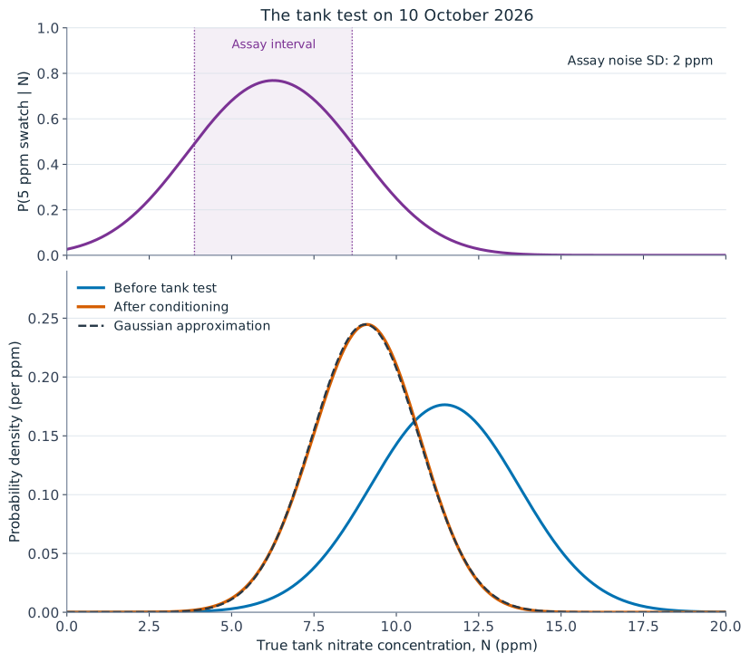
Figure 1. The tank test on the 10th of October. The upper panel shows the probability of obtaining the 5 ppm swatch at each possible true concentration. The lower panel shows the Gaussian prior, the posterior obtained by conditioning that prior on the category, and its Gaussian approximation. The posterior is exact for this incoming Gaussian prior and the assumed likelihood.

The posterior depends on both the prior and the likelihood. Assay noise allows a true concentration above the category boundary to produce the observed swatch. The updated mean therefore need not equal the number printed on the chart.

Calculating the update

With a Gaussian prior for the state, the predicted assay response is also Gaussian:

$$z^*\mid\mathcal D\sim\mathcal N(\mu_z,S), \qquad \mu_z=Hm^-, \qquad S=HP^-H^\mathsf{T}+\sigma^2.$$

Here $m^-$ and $P^-$ are the state mean and covariance immediately before the test.

Conditioning $z^*$ on the observed interval gives a truncated normal distribution, whose mean $\bar z$ and variance $v_z$ can be calculated analytically. Using these in the conditional Gaussian formulas gives the updated state moments:

$$K=\frac{P^-H^\mathsf{T}}{S},$$ $$m^+=m^-+K(\bar z-\mu_z),$$ $$P^+=P^-+KK^\mathsf{T}(v_z-S).$$

The vector $K$ determines how information about the assay response affects each state component. The mean update depends on the difference between the conditional assay mean and its prediction. The covariance update accounts for the uncertainty removed by learning which interval contains the response.

The category leaves uncertainty about the assay value within that interval. Retaining $v_z$ accounts for that uncertainty; inserting the swatch label as an exact assay value would discard it. If the continuous assay response were observed exactly, $v_z=0$ and these equations would reduce to the usual Kalman update.

These are exact posterior moments for the incoming Gaussian state distribution. The posterior itself is generally non-Gaussian. I replace it with the Gaussian having mean $m^+$ and covariance $P^+$, then use that approximation for the next prediction.

This replacement is the Gaussian assumed-density approximation.¹ It preserves the joint mean and covariance at this update. Subsequent updates start from the approximation, so the moments need not agree with those of the posterior obtained from the entire history.

Learning about the accumulation rate

For a tank test, the rate component of the mean update is

$$m_r^+-m_r^- = \frac{P_{rN}^-}{P_{NN}^-+\sigma^2} (\bar z-m_N^-).$$

A concentration measurement can therefore change the estimated rate when the prior covariance $P_{rN}^-$ is non-zero.

Physically, a higher accumulation rate tends to produce a higher concentration after some time has passed. If a new reading favours a lower concentration than predicted, some of that information can therefore pull the rate estimate down as well.

On the 6th of October, I recorded the 15 ppm tank swatch. On the 10th I recorded 5 ppm, followed by 15 ppm again on the 17th. In the replay, the tank test on the 10th produced the following update:

Quantity	Before the tank test	After the tank test
Tank nitrate, ppm	$11.47\pm2.26$	$9.06\pm1.63$
Net accumulation rate, ppm/week	$3.24\pm1.21$	$2.11\pm0.96$

The uncertainties here are one standard deviation. The “before” column already includes that day’s tap-water result; the table isolates the effect of the tank test.

It is particularly useful that one colour comparison can update both the concentration and its rate of change. The information about the rate comes from the covariance established by the dynamics. In this case, uncertainty in both quantities has also decreased.

Water changes also introduce relationships between tank and tap concentration. Consequently, a test can affect state components other than the one appearing directly in its likelihood. Keeping the full covariance matrix allows those relationships to be carried through the calculation.

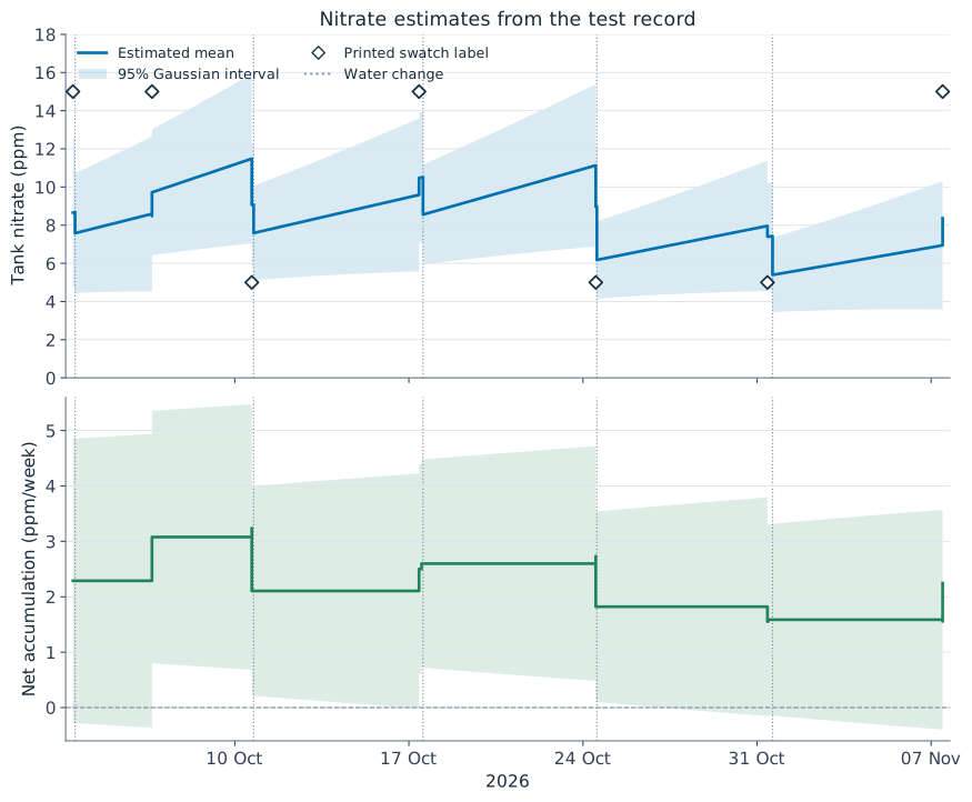
Figure 2. Filtering estimates from the replay, using only the records available up to each point. Lines show means and shading shows the Gaussian 95% marginal intervals, $m\pm1.96s$. Diamonds mark the printed tank-test labels, which are categories rather than exact concentration measurements. Dotted vertical lines mark water changes. The jumps at tests and interventions are part of the calculation; no smoothing has been applied.

The concentration forecast rises between tests when the estimated rate is positive, while its uncertainty grows. A test can change both the estimate and the uncertainty. A water change produces a separate jump in concentration.

The rate remains a net balance. A reduction could be consistent with increased plant uptake, but these data cannot separate that from reduced nitrate production or other changes.

Checking the Gaussian approximation

We can examine the effect of the repeated Gaussian approximations by replaying the same record with a bootstrap particle filter.² It represents the state distribution by weighted samples. Each sample is advanced through the dynamics and water changes, then weighted by the likelihood of the next observation. When the weights become concentrated, resampling gives more representation to the states supported by the observations.

The comparison used the same starting distribution, dynamics, assay noise and recorded observation intervals. For uncertain water-change fractions, the particle filter used beta distributions³ with the means and variances used by the GADF. This supplies a full distribution on fractions between zero and one, where the GADF moment calculation needs only the first two moments.

I replayed the record from the 13th of September to the 7th of November: 18 observations and seven water changes. There were three particle-filter runs, each with 200,000 particles and a different random seed.⁴

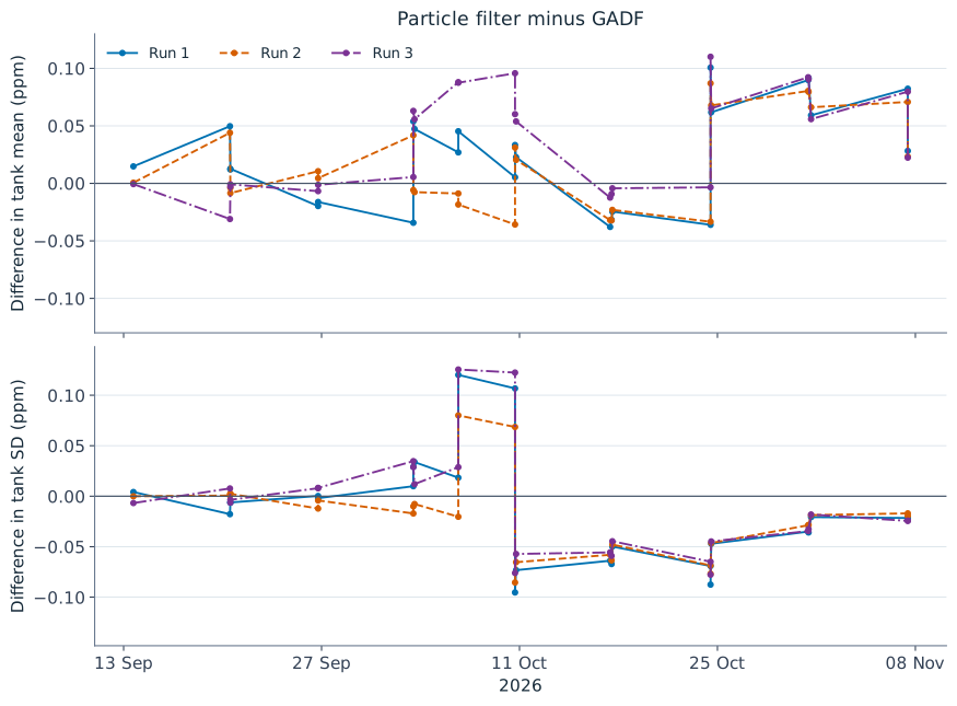
Figure 3. Particle-filter estimates minus GADF estimates after each recorded event. The upper panel compares tank concentration means; the lower panel compares their standard deviations. The three runs are shown separately. The differences include Monte Carlo sampling error as well as any effect of the Gaussian approximation.

Across all events and runs, the mean absolute difference in the estimated tank concentration was about 0.040 ppm; the largest was 0.110 ppm. The mean absolute difference in its standard deviation was about 0.039 ppm.

For this record, those differences are small compared with the uncertainty in the concentration estimates. The comparison supports using the GADF for these summaries over this period. It does not establish agreement in every tail probability, or tell us whether the physical and measurement assumptions describe the aquarium well.

I will look at the assay noise, category boundaries and predictive checks in the next post.

Footnotes

1. Simo Särkkä and Lennart Svensson (2023), Bayesian Filtering and Smoothing, second edition, Cambridge University Press, Chapter 8. The interval-observation update here uses the truncated-normal moments of the latent assay response. ↩

2. Särkkä and Svensson (2023), Bayesian Filtering and Smoothing, Chapter 11. ↩

3. Beta distributions were chosen because they constrain the replacement fraction between zero and one while matching the GADF’s assumed mean and variance; the choice of distribution family is an additional modelling assumption. ↩

4. Further runs and a check at larger particle counts would be needed to distinguish Monte Carlo error from the effect of the Gaussian approximation more reliably, but three is sufficient for a “quick look.” ↩